

Depth Estimation and 3D Mapping on Nvidia Jetson Nano
Python project.
The goal of this project is to build a robot capable of mapping its environment in a 3D simulation view. This article describes how to configure and use a Jetson Nano for a 3D mapping project where a neural network is used for depth estimation. The Jetson will also be connected to an Arduino Nano to get the gyro data from its IMU to project the depth values in a 3D world based on the orientation of the robot.
GitHub link: https://github.com/Apiquet/DepthEstimationAnd3dMapping
To achieve this project, the following steps will be performed:
- Configure the electronics board used on the robot (a Jetson Nano),
- Download a neural network for depth estimation in a tflite format from TensorFlow Hub and test it to verify its behavior and make the code to do inference on a livestream from USB camera (as this is going to be a big project, I choose to download a pre-trained tflite model to save time for all the other steps. However, in a future post, I will build a depth estimation neural network from scratch to replace this one),
- Configure an Arduino Nano to send the outputs of its IMU. Thanks to this IMU, we will be able to project the depth values in a 3D simulation view,
- Send the IMU data to the Jetson Nano from the Arduino,
- Create a part with Solidworks to fix the USD camera and the Arduino to the Jetson Nano,
- Build the 3D simulation to project the depth map based on the orientation of the IMU
Table of Contents
- Jetson Nano Setup
- Depth Estimation and TFLite
- Configure an Arduino to send the outputs of its IMU
- Get and parse Serial data on the Jetson Nano
- Create a part with Solidworks to fix the USD camera and the Arduino to the Jetson Nano.
- 3D simulation to project the depth map based on the orientation of the IMU
- Convert gyro to orientation
- Update robot’s orientation in a 3D view
- Depth map projection
- Projection of a 2D point in the real world
- Projection according to the orientation of the robot
- Project on specific orientations
- Projection of a real scene
- Rescale the depth map for better projection
- 3D scene
- Conclusion
1) Jetson Nano Setup
The Jetson Nano is an electronic board developed by NVIDIA for AI and robotics projects. It has a large computing capacity compared to its size, especially for AI.
The full setup tutorial can be found in the official website: https://developer.nvidia.com/embedded/learn/get-started-jetson-nano-2gb-devkit#prepare
The main steps will be formatting an SD card (at least 64go is recommended), and writing the Jetson Nano Image on it. The SD card. Then, the SD card can be inserted to the Jetson Nano and keyboard, mouse and a screen can be connected. The card will power on automatically after connecting an USB-C power supply.
A complete description of the board is available here.
2) Depth Estimation and TFLite
In the previous articles, I explained how to build from scratch a complete Deep Learning Framework only using numpy and how to implement a neural network to control a drone with hand signals. Then, I showed how to implement a complex neural network designed for object detection, how to train it and how to add module to do multi-object tracking (MOT). Finally, I described how to take and reuse its feature extractor to build different architectures designed for image segmentation and style transfer.
In this article, I decided to show how to build an application based on a neural network without having to design, implement and train it. We will simply download it from TensorFlow Hub, a great dataset of models. We will download the tflite version which is more efficient in term of size and power consumption. A next article will talk more about the advantage of TFLite and how to use it to optimize a model with quantization, quantization aware training, pruning, etc. TFLite-Macro also exists to deploy models on a microcontroller.
The chosen model can be found on TensorFlow Hub here. A code example is also provided to get inferences from a tflite model:
- Download the tflite model
- Create an interpreter from the saved model and allocate tensors
- Get input and output details (shape, type, etc.) to know the pre and post process will be needed
- Get the input image (a single image, images from a video, images from a livestream, etc.)
- Preprocess the input image to fit the model needs
- Send the data to the interpreter and get the inference
- Postprocess the inference to use and/or visualize the result
# 1: download the tflite model
TFLITE_FILE_PATH = 'model/midas_v2_1_small.tflite'

if not os.path.isfile(TFLITE_FILE_PATH):
    tflite_model_url = "https://tfhub.dev/intel/lite-model/midas/v2_1_small/1/lite/1?lite-format=tflite"
    urllib.request.urlretrieve(tflite_model_url, TFLITE_FILE_PATH)


# 2: create an interpreter from the saved model and allocate tensors
interpreter = tf.lite.Interpreter(model_path=TFLITE_FILE_PATH)
interpreter.allocate_tensors()

# 3: get input and output details
input_details = interpreter.get_input_details()
output_details = interpreter.get_output_details()

print(input_details)
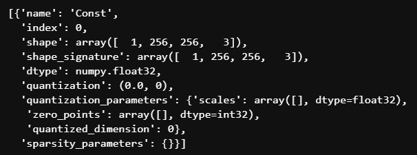
The input details shows the format of the image : [1, width, height, channels] and the format float32. According to the code example in the model page, we need to have an image in RGB format, then preprocess it to normalize it, resize it to 256×256 and add a dimension on the 0 index.
def preprocess_image(rgb_img, resize_shape):
"""
Function to preprocess an image
Normalization and resized to resize_shape
Args:
- (cv2 image) image in rgb format
- (numpy array) module_output : output of the model
- (int) legend_size: factor to multiply legend sized calculated
Return:
- (tf.Tensor) normalized and resized image in tensor
"""
normalized_img = rgb_img / 255.0
img_resized = tf.image.resize(normalized_img, resize_shape,
method='bicubic',
preserve_aspect_ratio=False)
img_resized = tf.transpose(img_resized, [2, 0, 1])
img_input = img_resized.numpy()
reshape_img = img_input.reshape(1, resize_shape[0], resize_shape[1], 3)
tensor = tf.convert_to_tensor(reshape_img, dtype=tf.float32)
return tensor
def postprocess_inference(img, module_output):
"""
Function to overlap segmentation map with image
Args:
- (cv2.image) Raw input image in RGB
- (numpy array) module_output : output of the model
- (int) legend_size: factor to multiply legend sized calculated
Return:
- (PIL image) overlap between img and module_output
"""
origin_height, origin_width, _ = img.shape
im_pil = Image.fromarray(img)
depth_min = module_output.min()
depth_max = module_output.max()
# rescale depthmap between 0-255
depth_rescaled = (255 * (module_output - depth_min) / (depth_max - depth_min)).astype("uint8")
depth_rescaled_3chn = cv2.cvtColor(depth_rescaled,
cv2.COLOR_GRAY2RGB)
# apply cv2.COLORMAP_RAINBOW for visualization
module_output_3chn = cv2.applyColorMap(depth_rescaled_3chn,
cv2.COLORMAP_RAINBOW)
module_output_3chn = cv2.resize(module_output_3chn,
(origin_width, origin_height),
interpolation=cv2.INTER_CUBIC)
seg_pil = Image.fromarray(module_output_3chn.astype('uint8'), 'RGB')
# overlap module_output on image
overlap = Image.blend(im_pil, seg_pil, alpha=0.6)
return overlap
# 4: get input image
img = cv2.imread('images/dog.jpg')
rgb_img = cv2.cvtColor(img, cv2.COLOR_BGR2RGB)
# 5: preprocess input image
input_data = preprocess_image(rgb_img, [256, 256])
# 6: get result
interpreter.set_tensor(input_details[0]['index'], input_data)
interpreter.invoke()
output_data = interpreter.get_tensor(output_details[0]['index'])
# 7: post processing to view results
output_data = np.squeeze(output_data, axis=0)
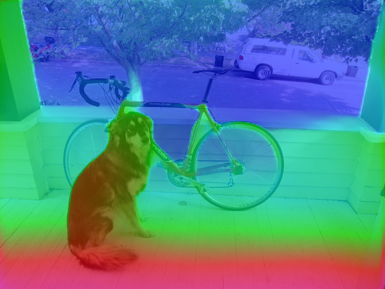
overlap = postprocess_inference(rgb_img, output_data)
overlap
Here is the result on the provided example on the model’s page:
We can also infer the model on a video:
# to reduce the output gif size,
# keep one frame every two and divide by two the resolution
keep_every=2
resize_fact=0.5
output_gif = "images/person_dog_depthEstimation_tflite.gif"

cap = cv2.VideoCapture("images/person_dog.mp4")
number_of_frame = int(cap.get(cv2.CAP_PROP_FRAME_COUNT))
imgs = []
for i in tqdm(range(number_of_frame)):
    if i%keep_every != 0 and keep_every != 1:
        continue
    _, image = cap.read()
    rgb_img = cv2.cvtColor(image, cv2.COLOR_BGR2RGB)

    # preprocess input image
    input_data = preprocess_image(rgb_img, [256, 256])

    # reshape data according to input_details
    input_data = tf.transpose(input_data, [0, 2, 3, 1])

    # Get result
    interpreter.set_tensor(input_details[0]['index'], input_data)
    interpreter.invoke()
    output_data = interpreter.get_tensor(output_details[0]['index'])

    # post processing
    output_data = np.squeeze(output_data, axis=0)
    overlap = overlap_img_with_segmap(rgb_img, output_data)
    overlap = overlap.resize((int(overlap.size[0]*resize_fact),
                                  int(overlap.size[1]*resize_fact)))
    imgs.append(overlap)

imgs[0].save(output_gif", format='GIF',
             append_images=imgs[1:],
             save_all=True, loop=0)
gif = imageio.mimread(output_gif, memtest=False)
imageio.mimsave(output_gif, gif, fps=30)

3) Configure an Arduino to send the outputs of its IMU
The Arduino Nano used in this project can be found on the official Arduino website here.
This Arduino has multiple embedded sensors :
“
- 9 axis inertial sensor: what makes this board ideal for wearable devices
- humidity, and temperature sensor: to get highly accurate measurements of the environmental conditions
- barometric sensor: you could make a simple weather station
- microphone: to capture and analyze sound in real time
- gesture, proximity, light color and light intensity sensor : estimate the room’s luminosity, but also whether someone is moving close to the board
“
We are going to use the 9 axis inertial sensor provided by the IMU to know in which direction the depth values have to be projected in the 3D simulation view. This IMU is composed of 3 elements:
- Accelerometer: measures changes in velocity,
- Gyroscope: measures changes in orientation and rotational velocity,
- Magnetometer: measures direction of the Earth’s magnetic field.
For the first version we will consider that the robot will be on the center of the room and will just turn around to map the entire room. In this case, we only need to get the gyroscope data to know the orientation of the robot at each frame (with integrations).
The following code example gets the magnetometer data from the Arduino and send it to the Serial port (to read it on the Jetson Nano. The gyroscope data can be obtained with IMU.readGyroscope(x, y, z).
#include <Arduino_LSM9DS1.h>

void setup() {
  Serial.begin(9600);
  while (!Serial);

  // Initialize IMU
  if (!IMU.begin()) {
    Serial.println("Failed to initialize IMU");
    while (1);
  }
}

void loop() {
  float x, y, z;
  if (IMU.magneticFieldAvailable()) {
      // get only magnetometer data
      IMU.readMagneticField(x, y, z);
      // send data in format x: x_value
      Serial.print("x:");
      Serial.print(x);
      Serial.print(' ');
      Serial.print("y:");
      Serial.print(y);
      Serial.print(' ');
      Serial.print("z:");
      Serial.println(z);
  }
}
In the Arduino IDE, we can verify that the data is sent from the Arduino with the Serial Monitor and Plotter:

The Serial Monitor allows us to verify the good format of the data:
x:19.34 y:23.01 z:-33.83
The Serial Plotter allows us to verify the good behavior of the data when we rotate the Arduino.
4) Get and parse Serial data on the Jetson Nano
To read the data from the Jetson Nano, the Arduino should be connected through an USB port and the serial python package will let us reach the data and parse it:
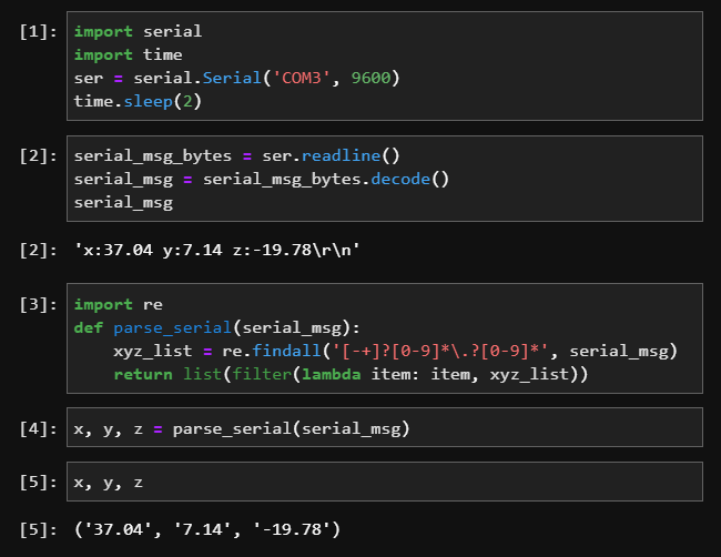
The simple code above parse the Serial input to get the data from the Arduino.
5) Create a part with Solidworks to fix the USD camera and the Arduino to the Jetson Nano.
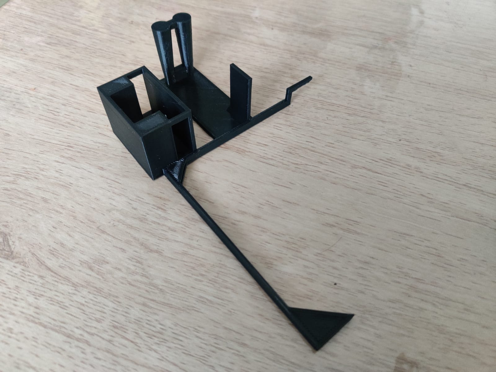
To ensure a good repeatability of my tests, I had to build a support to carry out the Jetson Nano, the USB camera and the Arduino. Plus, to have a good projection, I needed to have my rotation axis on the Arduino board (a complete Solidworks tutorial is available on my website here).
My final part is the following:
The green bar will by the rotation axis and the Arduino will be on the same axis:
Please note that I only did the pieces on the first animation: the Camera, the Arduino and the Jetson Nano comes from online resources that can be found here.
The following animations show how each part was built (a complete Solidworks tutorial is available on my website here):
The webcam and Arduino Support:
The cable management part:

The final assembly:
A short time-lapse of the 3D printing:
The rotation bar:

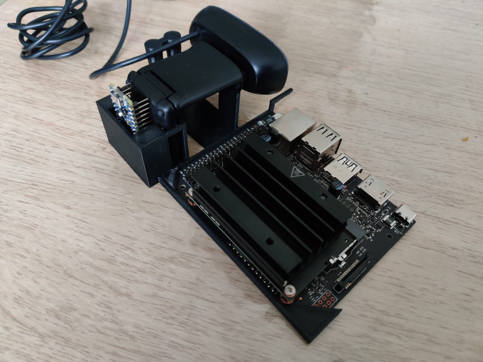
The final real result of the main part with the Jetson Nano, the webcam and the Arduino:

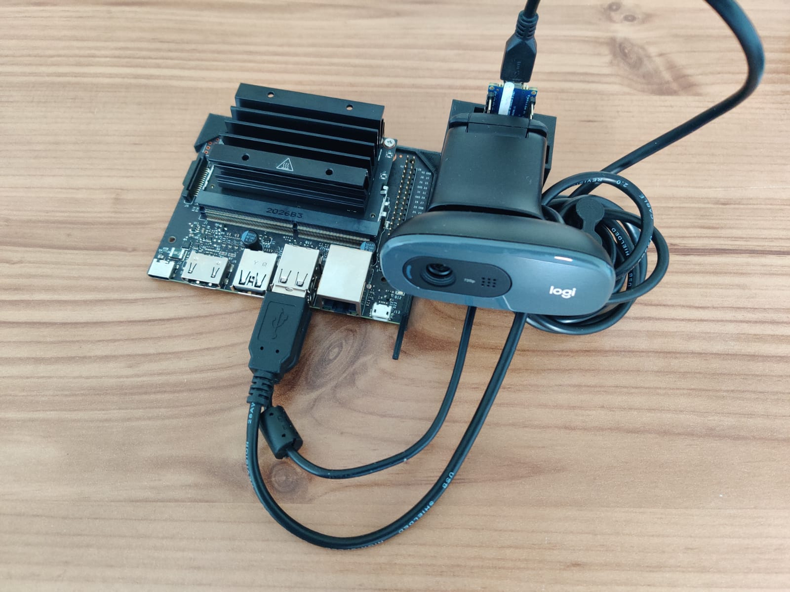
The final result after the cable management:
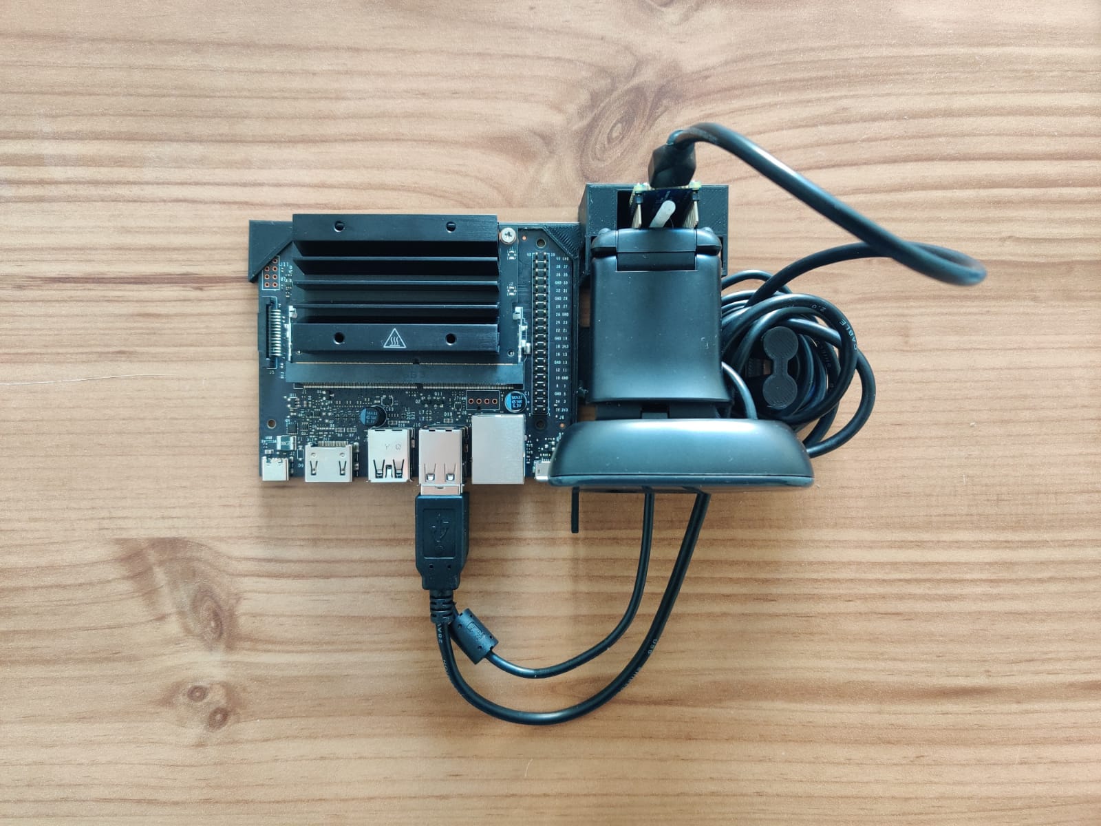
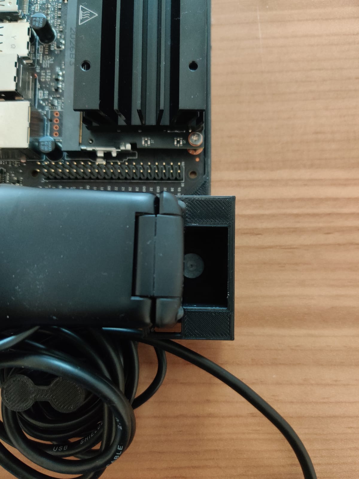
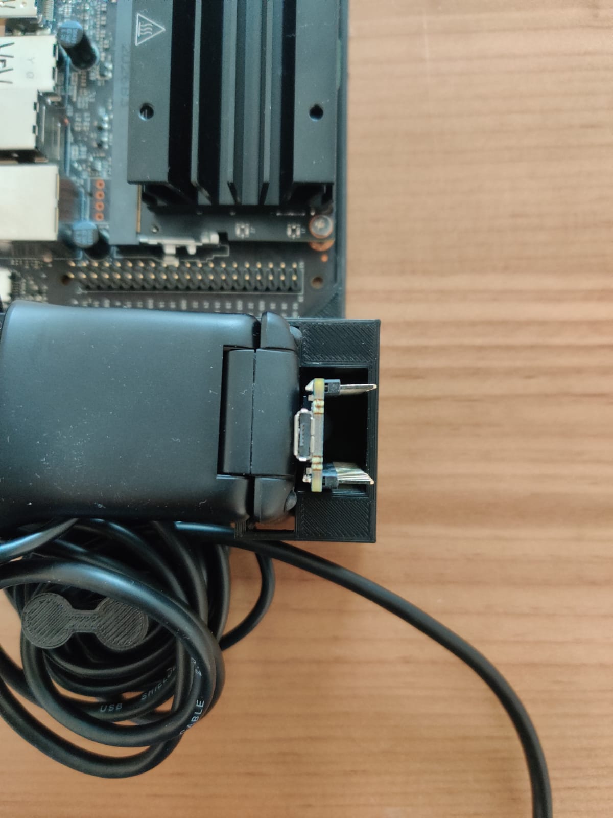
As mentioned at the beginning of the section: to have a good projection of my depth values, I needed to have my rotation axis on the Arduino board axis because I get my current angles from it. This is the case thanks to the rotation bar (the white bar with the Arduino board):
But the rotation axis is not exactly on the Arduino board, this causes the Arduino board to turn around the rotation axis. To fix this, I removed the bar to only keep its base and I turned the Arduino around. The next photos show how close the Arduino board is from the center of the rotation (the center of the white base):
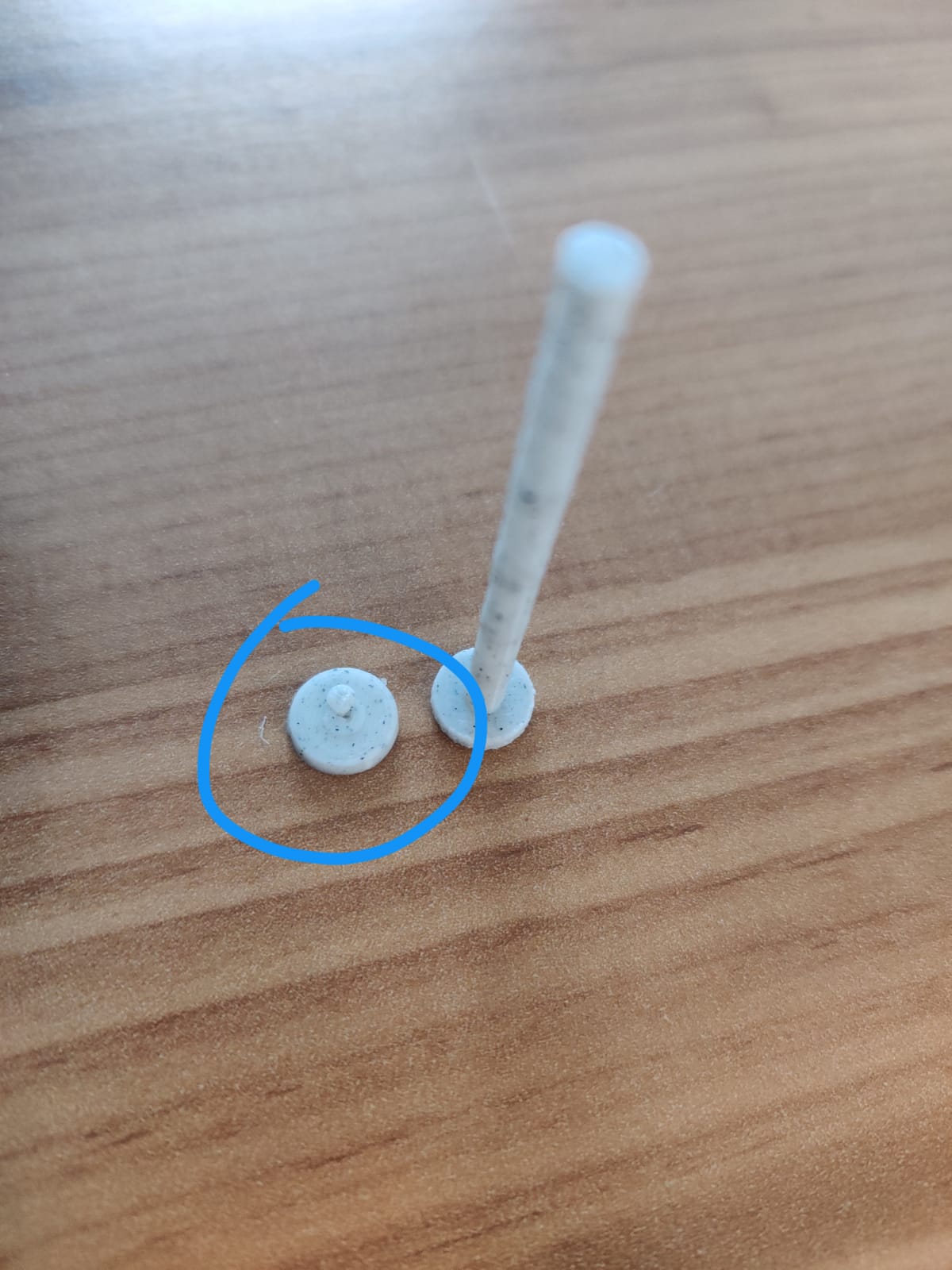
The rotation axis is now perfectly on the axis of the Arduino.
Note: as the cable management part was not big enough, I updated the solidworks model. I also remove the bar from the rotation base to only keep its base (the white circle clicked in blue):
6) 3D simulation to project the depth map based on the orientation of the IMU
6-1) Convert gyro to orientation
To project the depth values to the good direction in the 3D world, the first step is to integrate the gyroscope’s data from the IMU on the robot to get its orientation. Please note that in our case, we will only use the robot for a single 360° to map a room: for a longer application, the accelerometer will have to be used to adjust the gyroscope drift.
First, the code developed in Section 4 must be reused to obtain the gyro data and analyze it to obtain the x, y, z data. The orientation will be obtained from the integration of the gyro data obtained from the Serial buffer (Serial buffers the data to make sure we don’t miss any data). To read and update the current orientation, the best way is to use a thread: this thread will run in parallel to the main iteration, thanks to it, we will only need to read the global variable “orientation” to know the direction of the robot.
Note : as the Arduino rotate around its x axis, only the x data from the Gyroscope will be used.
The gyro data is expressed in degrees per second, so we need to know how much data we are getting per second. Once we know this, we can divide the data by the number of data per second to get the degrees covered by the robot. This information is given by the Arduino with : IMU.gyroscopeSampleRate() (data sending rate):
x_orientation = 0

# 119 got from Arduino with IMU.gyroscopeSampleRate();
gyroscope_sample_rate = 119

def UpdateOrientation(ser):
    """
    Function to integration the x data from the Gyroscope
    and update the global variable x_orientation with the new value

    Args:
        - (serial.Serial) serial to get the gyroscope data
    """
    global x_orientation

    while True:
        serial_msg_bytes = ser.readline()
        serial_msg = serial_msg_bytes.decode()
        dx, dy, dz = parse_serial(serial_msg)

        # The gyroscope values are in degrees-per-second
        # divide each value by the number of samples per second
        dx_normalized = dx / gyroscope_sample_rate;

        # remove noise
        if(abs(dx_normalized) > 0.004):
            # update orientation
            x_orientation = x_orientation - dx_normalized*1.25
            x_orientation = x_orientation%360

# run the thread to update the x orientation in real time
Thread(target=UpdateOrientation, args=(ser,)).start(
Then, a simple loop can be developed to visualize the result:
while True:
    plt.clf()

    # plot origin in blue
    plt.scatter(0, 0, s=100, c='b')

    # find position of the end of the needle
    # 0.1 far from origin in direction of the orientation
    distance = 0.1
    x_orientation_rad = math.radians(x_orientation)
    x_pos = math.cos(x_orientation_rad)*distance
    y_pos = math.sin(x_orientation_rad)*distance

    # plot line between both position with circles
    plt.plot([0, x_pos], [0, y_pos], 'ro-')

    plt.xlim([-distance, distance])
    plt.ylim([-distance, distance])
    plt.pause(0.1)
The above code gives the following result where the orientation seems to be well calculated:
6-2) Update robot’s orientation in a 3D view
Quick recap of the job done so far:
- Configuration of the Jetson to run our code,
- Arduino configuration to send the gyroscope data to the Jetson,
- Modeling of the robot structure to have the rotation axis on one of the Arduino axis to facilitate the projection of the depth values in a 3D world and put the USD camera directly on an Arduino axis,
- 3D printing of the design,
- Calculation of the orientation of the robot based on the integration of gyroscopic data,
- Verification of the calculated orientation
There are two major steps left:
- Build a simple 3D view to show the robot orientation
- Project points from a depth map in function of the orientation
The code to convert the previous plot into a 3D one is very similar, the main difference is the use of “projection=’3d'”:
fig = plt.figure()

while True:
    ax = fig.add_subplot(111, projection='3d')

    # plot origin in blue
    ax.scatter(0, 0, s=100, c='b')

    # find position of the end of the needle
    # 0.1 far from origin in direction of the orientation
    distance = 0.1
    x_orientation_rad = math.radians(x_orientation)
    x_pos = math.cos(x_orientation_rad)*distance
    y_pos = math.sin(x_orientation_rad)*distance

    # plot line between both position with circles
    ax.quiver(0, 0, 0, x_pos, y_pos, 0,
              length=distance, normalize=True)

    ax.set_xlim(-distance, distance)
    ax.set_ylim(-distance, distance)
    ax.set_zlim(-distance, distance)

    plt.show()
    plt.pause(0.1)
    plt.gcf().clear()
Which gives the following result:
6-3) Depth map projection
6-3-a) Projection of a 2D point in the real world
To project a 2D point into 3D coordinates, the first thing to understand is how to use the depth value. the following schema shows to calculation’s principal:
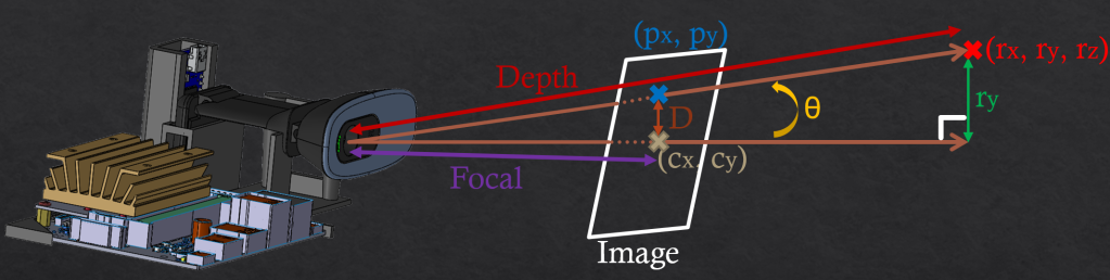
In the illustration above, we want to convert the 2D point (px, py) to the 3D point (rx, ry, rz) thanks to the depth value. To do so, we need to get the focal and the D value:
D_y = p_y – c_y
focal_y = image_height / (2*math.tan(v_fov/2))
With v_fov = vertical fov (can be found on the camera documentation)
We also know that:
tan(θ) = Opposite / Adjacent = D / focal
sin(θ) = Opposite / Hypotenuse = r_y / depth
Finally:
θ = atan[(p_y – c_y) / focal_y]
r_y = depth * sin(atan[(p_y – c_y) / focal_y])
Note: for x close to 0, atan(x)=x and sin(x)=x so in our case we could simplify the formula as r_y = depth * (p_y – c_y) / focal_y
The same calculation can be done for x (with horizontal fov instead of the vertical one)
With the above calculation, the projection was made in the camera referential but to have to position of the point in the real world we need to add the position of the camera. In our case, the camera is the origin so the camera position is (0, 0, 0).
The next part will be to use the robot orientation to project the point into the good direction,
6-3-b) Projection according to the orientation of the robot
As our robot is the origin of our referential and do a pure rotation around the x axis, we only need to rotate the projection around the x axis. To do so, we need to multiply the 3D point (px, py, pz) with a rotation matrix :
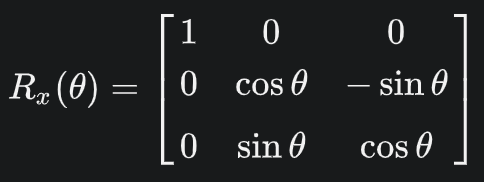
Here is the function that create the rotation matrix from a given angle:
def get_rotation_matrix(orientation):
    """
    Calculate the rotation matrix for a rotation around the x axis of n radians

    Args:
        - (float) orientation in radian
    Return:
        - (np.array) rotation matrix for a rotation around the x axis
    """
    rotation_matrix = np.array(
        [[1, 0, 0],
         [0, math.cos(orientation), -math.sin(orientation)],
         [0, math.sin(orientation), math.cos(orientation)]])
    return rotation_matrix
The following code do the projection of 1% of the depth:
def get_3d_points_from_depthmap(points_in_ned, depth_values,
                                depth_map, pourcentage_to_keep=1):
    """
    Project depth values into 3D point according to the robot orientation
    Uses global variable x_orientation

    Args:
        - (np.array) points_in_ned
        - (list) depth_values
        - (cv2 image) depth_map format (width, height, 1)
        - (int) pourcentage_to_keep: pourcentage of depth points to project
    Return:
        - (np.array) rotation matrix for a rotation around the x axis
    """
    for x in tqdm(range(image_width)):
        for y in range(image_height):

            # keep 0.1% of the points
            if random.randint(0, 999) >= pourcentage_to_keep:
                continue

            # get depth value
            x_depth_pos = int(x*x_depth_rescale_factor)
            y_depth_pos = int(y*y_depth_rescale_factor)
            depth_value = depth_map[x_depth_pos, y_depth_pos, 0]

            # get 3d vector
            x_point = depth_value * (x - c_x) / x_focal
            y_point = depth_value * (y - c_y) / y_focal
            point_3d_before_rotation = np.array([x_point, y_point, depth_value])

            # projection in function of the orientation
            point_3d_after_rotation = np.matmul(
                get_rotation_matrix(math.radians(x_orientation)),
                point_3d_before_rotation)
            points_in_ned = np.append(points_in_ned, point_3d_after_rotation)
            depth_values.append(depth_value)
    return points_in_ned, depth_values
After developing the code for the visualization part (available here), we were able to test the whole process of projection from a 2D images to a 3D scene:
- Load an arbitrary image
- Use the depth estimation model to get the depth values
- convert n% of random points to 3D points
- get the current robot orientation (fake it with an increment of x degrees to test a turnaround)
- rotate the 3D points wrt to the robot’s orientation
- create a colormap from blue to red to better visualize the depth
- create a 3D view with:
- the referential (x, y, z) in red, green and blue
- an arrow in black to visualize the robot orientation in real time
- all the 3D points with the colormap
In the above visualization, we can see that the points are projected along the good direction following the robot orientation (black arrow). Everything seems to work fine, we can now move on real tests.
6-3-b) Project on specific orientations
There is no need to continuously project the camera on real time, it will just add new data on the previous ones and make the simulations very noisy. A first approach is to pre configure orientations to do. In our case, I choose to do a projection every 60°:
DEGREES_INTERVAL = 60

ORIENTATIONS_DONE = []
ORIENTATIONS_TODO = [orientation for orientation
                     in range(0, 359, DEGREES_INTERVAL)]
We then need to check in the projection if we are around an orientation to do. If this is the case, we project the current depth map into the simulation and we move the orientation to the orientations done list. We can also display the orientations done in green and the ones to do in red. In the following example, we projected the depth map on the initial orientation 0° and we started the rotation of the robot to reach the 60°:
We can notice that the orientation 0° was done so the arrow 0° is now in green, the others are still in red. Then we can do all orientations:
7) Projection of a real scene
7-1) Rescale the depth map for better projection
After some experiments with the depth estimation model, we can notice that it determines the perspective between objects well but not the actual distance. To solve this problem, we can ask the user to give the minimum and maximum distances seen by the camera and we can resize the depth map according to these distances. To do this, we need to show the current image and the generated depth map to the user and request the minimum and maximum distance values.
Note: the red/green arrows (the target orientations) were also moved to another display for clarity.
7-2) 3D scene
Finally, the following illustration is the projection of a hall (harder than a simple room):

Explanation of the 3D scene:

From the point of view of the robot, it cannot see the black part so it stayed empty in the 3D scene. We can also notice that the angle of the hinges (number 1) was also mapped. We got a good angle for the door in orange (between number 1 and 2). The rest of the hall is recognizable but the walls are a bit curved instead of straight.
Conclusion
In previous articles, we implemented neural networks for computer vision and reinforcement learning. Here, we have addressed a way to deploy a neural network on a concrete task to solve a real-world problem.
In particular, we learned:
- How to configure electronics boards (a Jetson Nano and an Arduino Nano),
- How to connect electronics board in Serial communication to send the IMU information from the Arduino to the Jetson
- How to download a neural network for depth estimation in a tflite format from TensorFlow Hub and how to verify its behavior,
- How to use the depth map values, position and the IMU data to project points in a 3D simulation view representing the real world,
- How to build a part with Solidworks that fits our needs,
- How to build a 3D simulation view to project 3D points
I hope this helps others.
Here you can find my project:
https://github.com/Apiquet/DepthEstimationAnd3dMapping
